An Overview of Tabnet - Tabular Data Deep Learning
Hey guys! I've been exploring the tabnet model for a few days since stumbling upon it in a Github repo. For the sake of the this post, I would just like to put down in words my understanding of the model to help you and I better understand it.
First and foremost, I would like to credit Francesco Pochetti for the images and symbolic dictionary from his blog post on Tabnet. I would also like to point you in the direction of the paper and Dreamquark's Github repo that has the model implemented in Pytorch.
With that being said, we could probably start with an initial overview of the model with the image below:
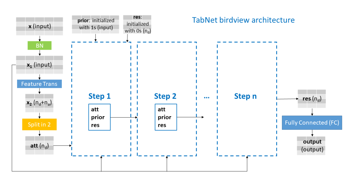
To understand what we're looking at, we can reference the dictionary provided:

As well as noting that:
BS -> batch size
input -> shape of the input dataset, e.g. number of features passed to the model.
n_d -> size of the decision layer, e.g. input features are mapped to n_d (where n_d<input) in Fully Connected (FC) layers.
n_a -> size of the attention bottleneck, e.g. input features are mapped to n_a (where n_a<input) and then to input again, giving the model a chance to learn which attributes to focus on.
Now, we could focus on the first part of the model:
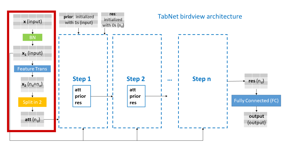
BN - Batch Normalization
The first part to notice is that we have the input that leads to "BN" or the batch normalization component.
Batch normalization can be understood through this mathematical pseudo-code:
    def batch_norm_math(self, X):
        # For batch B of size m
        μᵢ = (1/m)Σₘ xᵢᵐ            # Mean per feature
        σ²ᵢ = (1/m)Σₘ(xᵢᵐ - μᵢ)²    # Variance per feature
        x̂ᵢ = (xᵢ - μᵢ)/√(σ²ᵢ + ε)   # Normalized features

        return x̂ᵢ
Essentially, you could think of manipulating the data to mitigate extremes among other characteristics in the input dataset.
Also, the reason why we use the word "batch" is because a batch of data is sent to the model as input.
Feature Trans - Feature Transformer
After the normalized data is created, it gets fed into the feature transformer which can be understood it through the following image:

And, to then understand the first part of the feature transformer (the GLU layer), we can understand it through this image:

This could then be understood through this mathematical pseudo-code:
    def step_by_step(self):
        # 1. Linear Transformation
          W ∈ ℝᵈˣ²ᵐ (d: input dim, m: output dim)
          x ∈ ℝᵇˣᵈ (b: batch size)
          h = xW

        # 2. Batch Normalization
          μ = (1/B)Σᵢ hᵢ
          σ² = (1/B)Σᵢ(hᵢ - μ)²
          ĥ = (h - μ)/√(σ² + ε)

        # 3. GLU
          Split ĥ into ĥₜ and ĥg
          output = ĥₜ ⊙ σ(ĥg)
The Decision Step - A Decision Tree Like Component
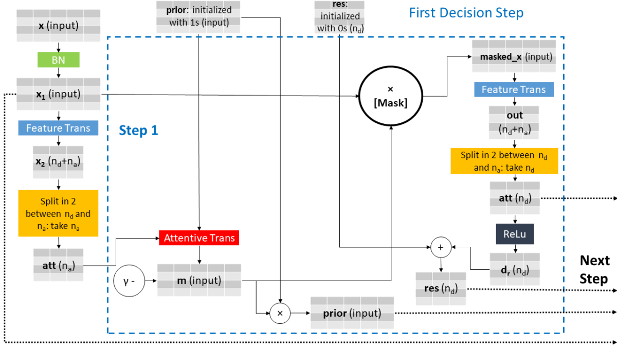
With these components of the model now roughly understood, the last part that it is essential to knowing how Tabnet works is by looking at the decision step.
Within this part, there is:
-
the mask
-
the attentive transformer
The Mask
You can think of the mask as a matrix that filters out what's unimportant. This also allows us to see which features Tabnet focuses on for each prediction (since it has instancewise feature selection); meaning that the model is also then very interpretable.
Here's an example you can run that shows what I mean.
The Attentive Transformer
The attentive transformer is what allows the model to focus on the different features through the iterative cycle of training. How it's set-up can be observed by the following image:

All of these components together create an output for each decision that are then all added together to make a decision.
How A Prediction is Made After All the Decision Steps
After the whole step process that's done, all the outputs from each of the steps are added together.A fully conneted layer is then applied for regression or a fully connected layer and then a softmax function are then applied to get a class prediction. All of this can be seen in the mathematical pseudocode below.
def tabnet_prediction_math(self, decision_steps):
    # dᵢ represents output from decision step i
    # Sum all decision step outputs into final hidden representation
    h = Σᵢ dᵢ

    # For Classification:
    # W is the weight matrix of final layer
    # b is the bias term
    # zⱼ is the logit for class j
    z = Wh + b                     # Linear transformation to C classes

    # pⱼ is probability for class j
    # C is the number of classes
    pⱼ = exp(zⱼ)/Σₖexp(zₖ)        # Softmax for class probabilities

    # ŷ is the final prediction (class label)
    ŷ = argmaxⱼ(pⱼ)               # Final class prediction

    # For Regression:
    # ŷ is the final prediction (regression value)
    # W is the weight matrix of final layer
    # b is the bias term
    ŷ = Wh + b                     # Linear transformation is final prediction

    return ŷ
In my next post, if you guys are interested, I can then go through how Tabnet trains itself on the data and its respective unsupervised pretraining characteristics.